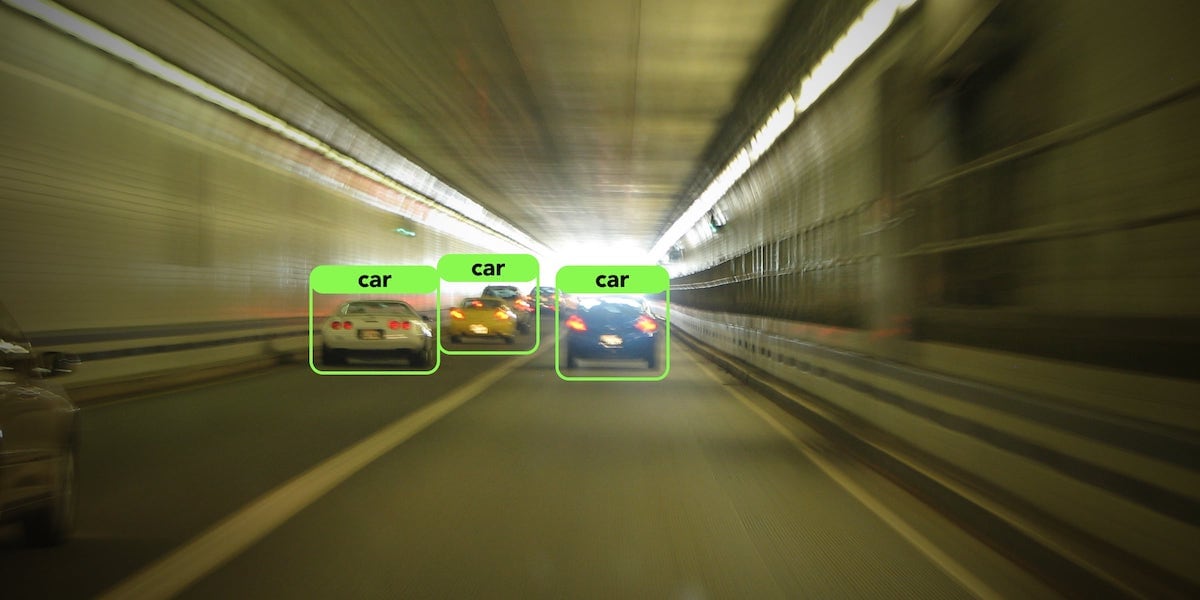
I just wrapped up a challenging computer vision project and have been thinking about lessons learned. Before we started the project I looked for information about what was possible with the latest technology. I wanted to know what sort of accuracy (precision and recall) I could expect under various conditions. I understand that every application is different, but I wanted at least a rough idea. I didn’t find the type of details that we needed, so we approached the problem in a way that would give us flexibility to change our approach with minimal rework. We used the Tensorflow Object Detection API as the main tool for creating an object detection model. I wanted to share, in general terms, some of the things which we discovered. My goal is to give someone else who is approaching a computer vision problem some information which may help guide their choices.
The customer’s objective was to get an inventory of widgets sitting on a rack of shelves. The widgets were fairly large and valuable, but for various reasons RFID and other radio based solutions were not an option. So, that is where computer vision came in. Using computer vision to solve this problem was not going to be an easy task. There were many obstacles to overcome, and I will discuss them in turn.
The first obstacle which had to be overcome was simply finding a place to mount cameras. The cameras had to be attached directly to the widget rack, and we needed to maximize the number of widgets visible per camera. The racks could have 3 to 4 shelves, each holding from 2 to 5 widgets across and 1 to 2 widgets deep. There were other racks with additional constraints, but we ignored them in favor of concentrating our efforts on the most common scenarios. After experimenting with several locations, the location which maximized field of view while limiting the number of cameras required was the side of the rack.
The main problem with placing tha cameras in this location had to do with simple geometry. The shelves were designed to efficiently hold widgets, not to make them visible. So, when viewing the widgets from the side the only portion which is reliably visible was the top. Fortunately, all the distinguishing characteristics of a widget are on the top, so they would theoretically be visible to a side-mounted camera. However, a problem occurs when cameras are oriented in such that they are facing vertically but capturing objects located on a horizontal plane. The data from the horizontal plane is project onto the vertical plane created by the cameras sensor.
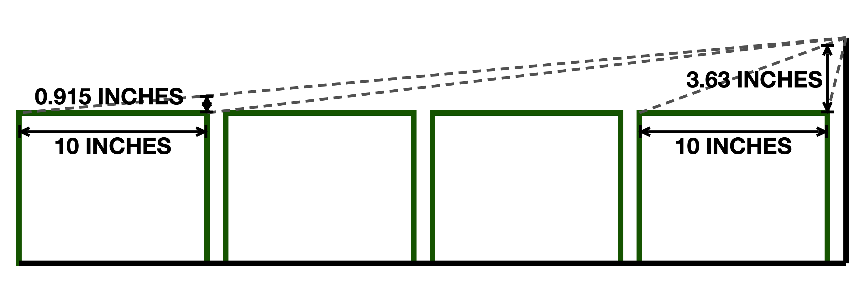
The projection is not in itself a problem, but it quickly becomes one as the horizontal distance between the camera and objects on the horizontal plane increases. In this specific case there was at most 4 inches from the top of the widgets to the bottom of the next shelf, except for on the top shelf, of course. This left little room to orient the cameras so that they were not facing parallel to the horizontal plane. In this configuration the further away on object is, the more the information that it displays is compressed into a smaller visible area.
This perspective effect is present regardless of camera position, and no other position was economically available to reduce this. The two widgets closest to the camera were reliably visible given the limited vertical distance. Placing the cameras on the back of the rack could have helped to mitigate the problem, but the number of cameras required would have blow the per rack budget. We were able to place additional cameras on the opposite side of wider racks, though this lead to the same widget potentially being visible in multiple photos. Identifying widgets which should not be included in the inventory was a general concern, so we committed to adding a post-processing step which would reconcile any potentially double-counted or non-relevant widgets.
Having dealt with the question of where the cameras would be located, we were able to move on to the next phase. We needed to gather enough images to train a computer vision model, but we were not sure exactly how many would be required. Since capturing images and classifying them is time consuming, we decided to start with a low number and add training examples as needed.
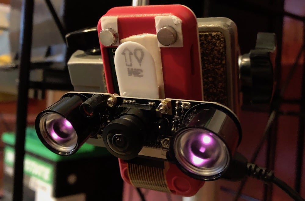
We mounted cameras in the rack and began capturing pictures of each type of widget. All of the widgets are roughly the same size and shape, they were all rectangular prisms (box shaped). Every widget was labeled, but the most prominent label was on the front, which was normally not visible. Fortunately, they all had some sort of distinguishing features. Or so we thought.
After our initial trials we discovered that one specific type of widget may come in different variations. That alone is not a show stopper, we could train to identify each specific version. The problem came when we found that some versions of a specific type of widget looked exactly like another type of widget. The only physical difference between the widget types was the labels they bore. So, we had to group some widget types together.
None of these complications prevented us from training a computer vision model. However, they did change what we could realistically expect the computer vision model to accomplish. It would simply not be possible to distinguish between certain types of widgets, and that impacts the ultimate goal of getting an accurate inventory. We proceeded knowing that we would need to find some way to augment the results of the computer vision process.
The first model we trained consisted of 18 classes with 86 examples per class. The examples were split into a training set with 70 images per class and an evaluation set with 16 images per class. The initial results looked amazing — too amazing. The overall mean average precision was 99%. We have scripts which automatically take source images and randomly split them into training and evaluation sets. Those scripts were used to create new training and evaluation sets with the same number of images per class, but composed of different images. The results of the additional runs mirrored the results of the first run.
In addition to training and evaluation sets we have a completely separate set of data for validation. This set consists of images taken in exactly real-world conditions. The training images were taken in near-real-world conditions. Because we need to gather so many images, we use some techniques to make capturing images easier, and this means that they don’t exactly reflect the real world. Also, the validation set is ran using the same inference engine which would be used in the final product. That allows us to also verify that the inference engine is working properly.
When we exported the models and ran them against the validation set, we found a much lower accuracy than the mean average precision (mAP) reported from the evaluation. We validated the accuracy to between 4 and 12 percent. When we looked at the bounding boxes which were predicted for the validation set, we noticed that they were way off. So, we decided an easy thing to try was changing out the architecture.
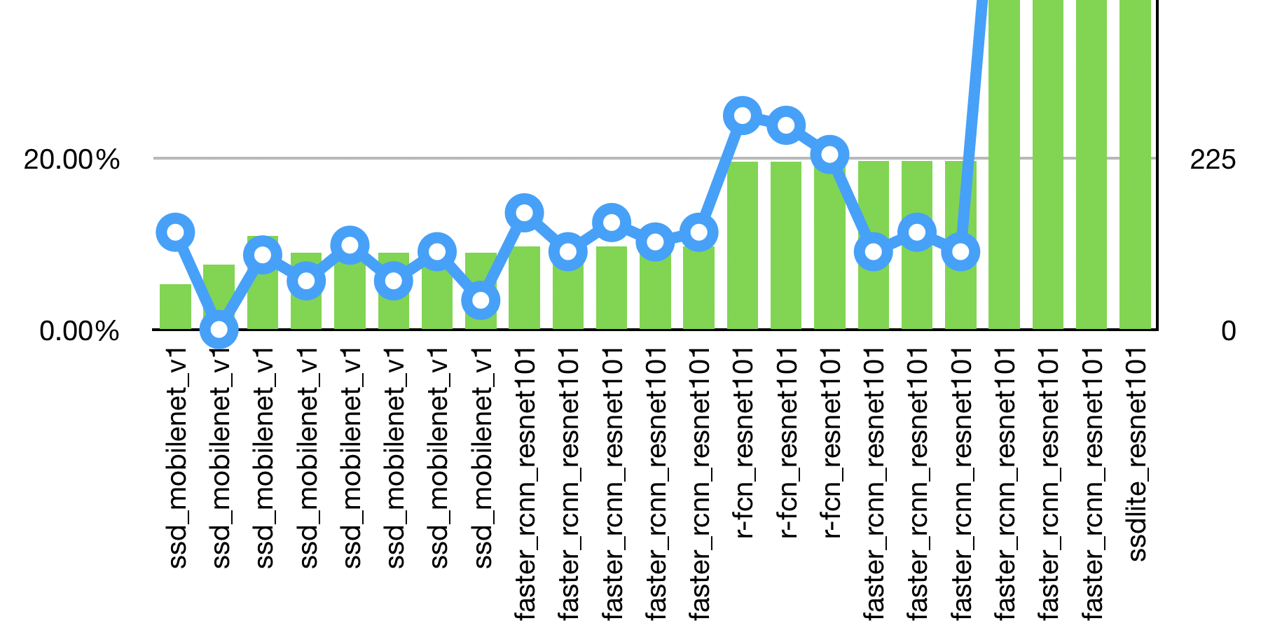
Since the intent was to push the inference to the edge (inference will be performed on a small IoT-type device), we originally did transfer learning based upon a SSD Mobilenet model. I knew that if we took advantage of a region proposal network we could get better bounding box performance. We switched to basing training off of a Faster R-CNN Resnet 101 model. This architecture yielded much better bounding box performance and a lot fewer false positives, but the validated accuracy was not where we needed it to be. It was only between 9 and 14 percent.
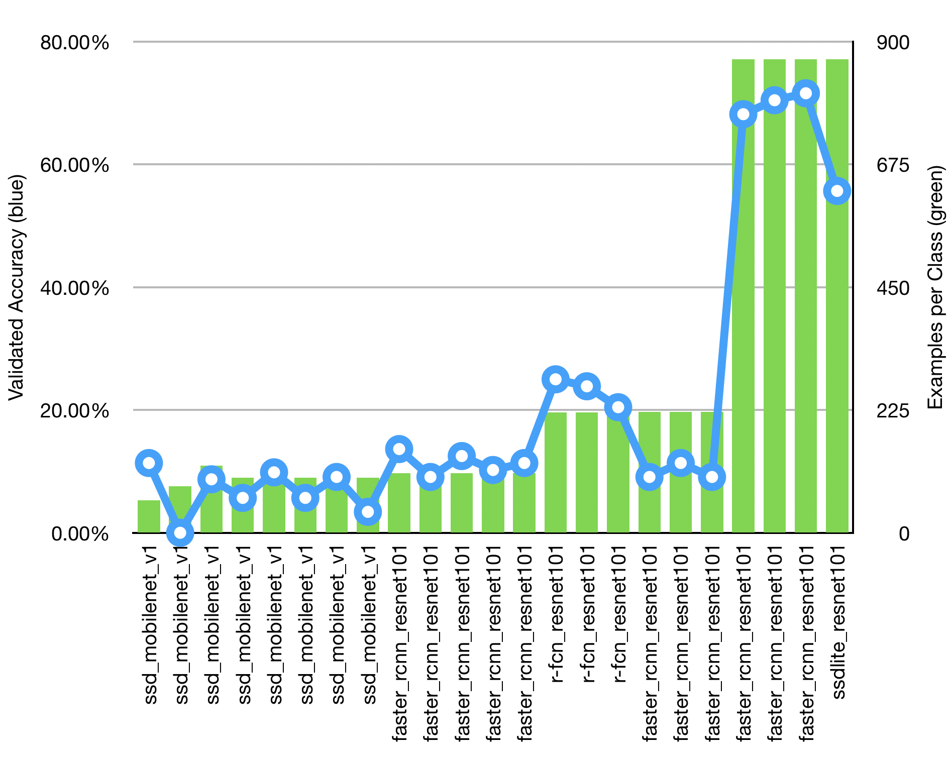
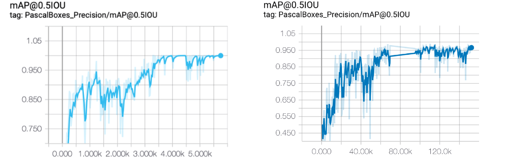
So, it seemed that we would need a lot more example images. To test that theory we increased the size of our data set to 220 images. The training set got 180 images per class and the remaining 40 images were used for evaluation. The best mean average precision of the evaluation set dropped to around 96 percent. The validate accuracy increased to 20-25 percent. That isn’t great, but it is nearly double what we were previously seeing.
I had also switched the basis model to one which used a Region-based Fully Convolutional Network. So, to fairly compare the results back to previous results, we reran the training using the Faster R-CNN Resnet 101 model. That model progressed just as the previous model. We didn’t fully train the Faster R-CNN model, but it’s performance was following the curve of the R-FCN based model, so we decided that drastically increasing the number of example images was required.
Based upon what we were seeing, we estimated that we would need at least 1000 images per class to get to a high accuracy model. By this time the number of classes we were working with had doubled, so it seemed that we needed to capture and tag at least 36,000 images. Quickly we decided to capture half that many and use image augmentation for the other half. Still, 18,000 images is a lot of images. We needed a strategy.
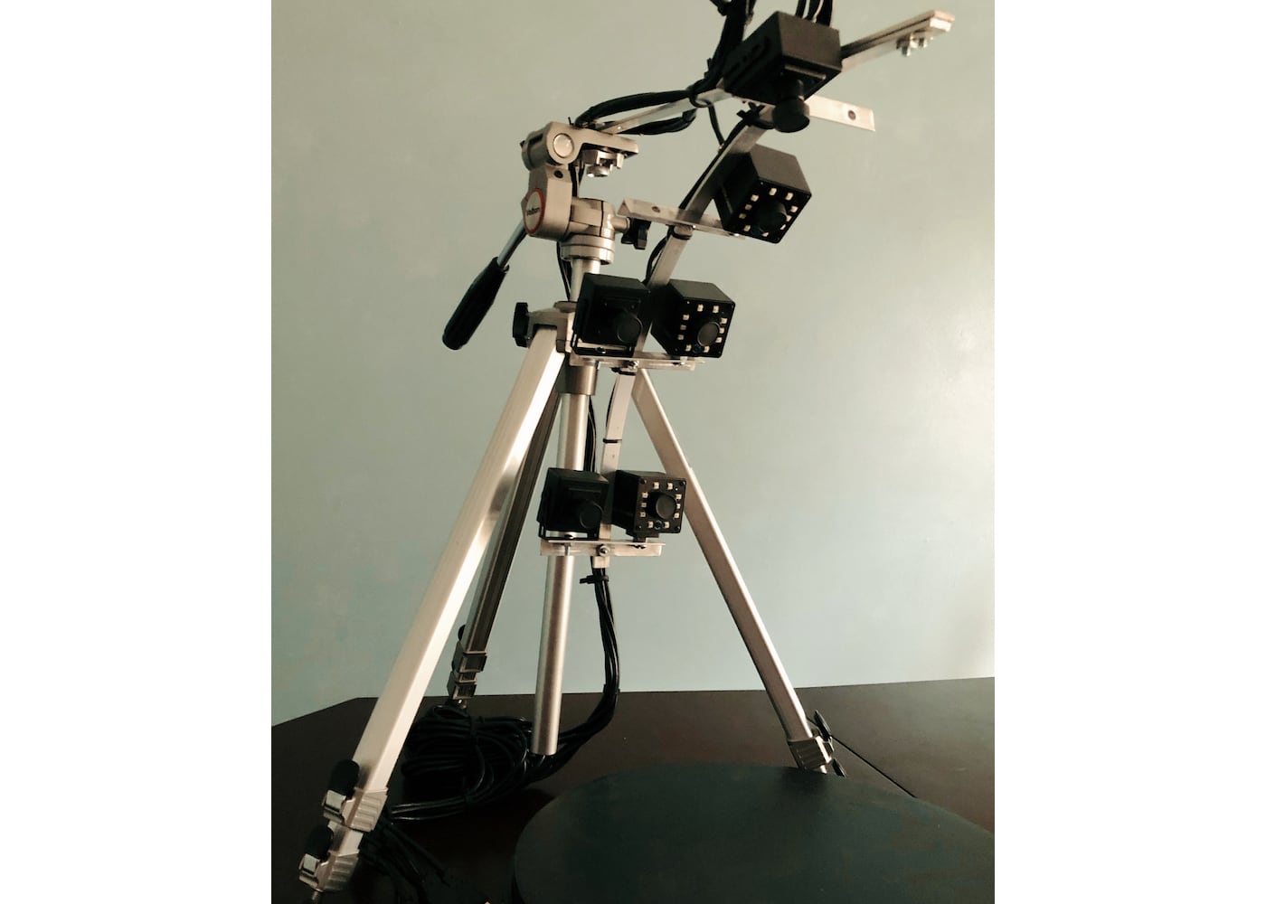
We grabbed a tripod, a powered USB hub, 8 spare cameras, some aluminum stock, bolts, and lots of zip ties. From those items we created a rig to capture images at various angles. We added an automatic turn table and a small python script. We had everything we needed to capture a lot of images relatively efficiently.
Even with the rig, it took two full days to capture just under 16,000 images (1000/hour). It took over a week and a half to tag the images (240/hour). At the end of the process we had 860 images per class, which was short of our goal, but we needed to meet a deadline. The important thing was seeing promising results, which we got. With 680 training images and 180 evaluation images per class, we ended up with a validated accuracy of 70 percent.
We had made some amazing progress on a very challenging problem, but there were still many problems left to solve. To this point we have completely ignored things such as partial obscured views. I should clarify, we expect the widgets to normally be partially obscured; only the top is visible. The ability to recognize and individual widgets decreases as the top of the widget becomes obscured. This could happen if something was placed on a widget or if a near widget is taller than a distant widget.
As a long shot we also looked at applying barcodes to the widgets. Linear barcodes applied to the top were basically useless. QR Codes worked when they were at least 4 inches square. And, they only worked for the closest 2 widgets due to the problems of perspective we described above. Finally, we directly attacked the problem of projecting data from one plane to another. We created a tall linear barcode, flipped it on its side, wrapped it around a dowel, and placed it so that it stuck up perpendicular from the top of the widget. The sideways barcodes (the lines running horizontally) could be recognized regardless of angle. However, they became unrecognizable at a distance, under low lighting conditions, and when there was image blur.
Given all of the challenges which remained on this project, it was unlikely that we would be able to get the level of accuracy which the client required, at least not while staying within their per rack budget constraints. So, the project was shelved, for now. As the price of small high-quality cameras fall, the cost to implement a computer vision based inventory system will also fall. At some point in the future it will become viable, even given all of the constraints.